Python for Finance – Stock Analysis & Portfolio Optimization Guide

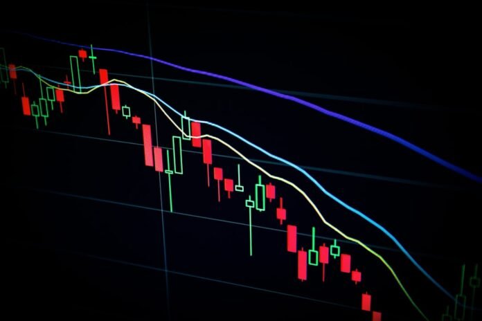
Python has become the dominant language in quantitative finance. From hedge funds to retail investors, Python powers stock screening, portfolio optimisation, risk modeling, and algorithmic strategy backtesting. This guide shows you the essential financial data science toolkit.

Downloading Stock Data with yfinance

pip install yfinance pandas numpy matplotlib scipy

import yfinance as yf
import pandas as pd

# Download OHLCV data
nifty50 = yf.download("^NSEI", start="2023-01-01", end="2026-08-01")
reliance = yf.download("RELIANCE.NS", start="2023-01-01", end="2026-08-01")

# Multiple tickers at once
tickers = ["RELIANCE.NS", "TCS.NS", "INFY.NS", "HDFCBANK.NS", "ICICIBANK.NS"]
prices  = yf.download(tickers, start="2023-01-01", end="2026-08-01")["Close"]

print(prices.tail())

Computing Returns and Statistics

import numpy as np

# Daily returns
returns = prices.pct_change().dropna()

# Annualised statistics (252 trading days/year)
TRADING_DAYS = 252

annual_return = returns.mean() * TRADING_DAYS
annual_vol    = returns.std() * np.sqrt(TRADING_DAYS)
sharpe_ratio  = annual_return / annual_vol

stats = pd.DataFrame({
    'Annual Return (%)':  (annual_return * 100).round(2),
    'Annual Volatility (%)': (annual_vol * 100).round(2),
    'Sharpe Ratio':       sharpe_ratio.round(2),
}).sort_values('Sharpe Ratio', ascending=False)

print(stats)

Technical Indicators

import pandas as pd

def add_technical_indicators(df):
    close = df['Close']

    # Moving averages
    df['SMA_20'] = close.rolling(20).mean()
    df['SMA_50'] = close.rolling(50).mean()
    df['EMA_12'] = close.ewm(span=12).mean()
    df['EMA_26'] = close.ewm(span=26).mean()

    # MACD
    df['MACD']        = df['EMA_12'] - df['EMA_26']
    df['MACD_Signal'] = df['MACD'].ewm(span=9).mean()
    df['MACD_Hist']   = df['MACD'] - df['MACD_Signal']

    # RSI
    delta = close.diff()
    gain  = delta.where(delta > 0, 0).rolling(14).mean()
    loss  = (-delta.where(delta < 0, 0)).rolling(14).mean()
    rs    = gain / loss
    df['RSI'] = 100 - (100 / (1 + rs))

    # Bollinger Bands
    df['BB_Mid']   = close.rolling(20).mean()
    df['BB_Upper'] = df['BB_Mid'] + 2 * close.rolling(20).std()
    df['BB_Lower'] = df['BB_Mid'] - 2 * close.rolling(20).std()

    return df

df = add_technical_indicators(reliance)

Modern Portfolio Theory – Efficient Frontier

from scipy.optimize import minimize

def portfolio_stats(weights, returns, cov_matrix):
    port_return = np.sum(returns.mean() * weights) * TRADING_DAYS
    port_vol    = np.sqrt(weights @ cov_matrix @ weights) * np.sqrt(TRADING_DAYS)
    sharpe      = port_return / port_vol
    return port_return, port_vol, sharpe

n_assets    = len(returns.columns)
cov_matrix  = returns.cov() * TRADING_DAYS

# Monte Carlo simulation of random portfolios
n_portfolios = 5000
results = np.zeros((n_portfolios, 3))
all_weights = []

for i in range(n_portfolios):
    w = np.random.dirichlet(np.ones(n_assets))  # random weights summing to 1
    r, v, s = portfolio_stats(w, returns, cov_matrix)
    results[i] = [r, v, s]
    all_weights.append(w)

results_df = pd.DataFrame(results, columns=['Return', 'Volatility', 'Sharpe'])

# Find maximum Sharpe ratio portfolio
best_idx = results_df['Sharpe'].idxmax()
best_weights = all_weights[best_idx]
print("Optimal weights:")
for ticker, w in zip(tickers, best_weights):
    print(f"  {ticker}: {w:.1%}")

Simple Backtesting – Moving Average Crossover

def backtest_sma_crossover(prices, short=20, long=50, initial_capital=100000):
    df = prices.to_frame('price')
    df['SMA_short'] = df['price'].rolling(short).mean()
    df['SMA_long']  = df['price'].rolling(long).mean()

    df['signal'] = 0
    df.loc[df['SMA_short'] > df['SMA_long'], 'signal'] = 1  # long
    df.loc[df['SMA_short'] < df['SMA_long'], 'signal'] = -1 # short

    df['returns']    = df['price'].pct_change()
    df['strategy']   = df['signal'].shift(1) * df['returns']

    df['cumulative_market']   = (1 + df['returns']).cumprod() * initial_capital
    df['cumulative_strategy'] = (1 + df['strategy']).cumprod() * initial_capital

    total_return = df['cumulative_strategy'].iloc[-1] / initial_capital - 1
    buy_hold     = df['cumulative_market'].iloc[-1] / initial_capital - 1

    print(f"Strategy return:  {total_return:.1%}")
    print(f"Buy & hold return: {buy_hold:.1%}")
    return df

result = backtest_sma_crossover(reliance['Close'])

Risk Metrics – Value at Risk and Max Drawdown

# Value at Risk (VaR) — 95% confidence
portfolio_returns = returns @ best_weights
VaR_95 = np.percentile(portfolio_returns, 5)
print(f"Daily VaR (95%): {VaR_95:.2%}")
print(f"On ₹10L investment, max daily loss (95% confidence): ₹{abs(VaR_95)*1000000:,.0f}")

# Maximum Drawdown
cumulative = (1 + portfolio_returns).cumprod()
rolling_max = cumulative.cummax()
drawdown    = (cumulative - rolling_max) / rolling_max
max_drawdown = drawdown.min()
print(f"Maximum Drawdown: {max_drawdown:.2%}")

Disclaimer

This guide is for educational purposes only. Nothing here constitutes financial advice. Past performance does not guarantee future returns. Always consult a SEBI-registered financial advisor before making investment decisions.

Conclusion

Python gives you a complete quantitative finance toolkit: yfinance for data, pandas for manipulation, scipy for optimisation, and matplotlib for visualisation. Understanding how to compute returns, build an efficient frontier, backtest simple strategies, and measure risk with VaR and drawdown are foundational skills for any data scientist working in finance. The code in this guide is a starting point — real trading systems require much more rigorous backtesting, transaction cost modeling, and risk management.