Modern data rarely follows a single simple pattern. In many real-world problems, data points come from multiple underlying processes, each contributing to the overall distribution. Traditional clustering or statistical methods often fail to capture this complexity. This is where probabilistic models become essential.
A Gauss mixture model provides a flexible and mathematically sound way to represent such data. Instead of assuming that all observations belong to one distribution, it models data as a combination of several Gaussian distributions. This approach enables more accurate clustering, density estimation, and pattern discovery.
In machine learning, statistics, and data science, this model plays a crucial role in unsupervised learning tasks where labels are not available.
Understanding Probabilistic Modeling
Before diving deeper, it is important to understand probabilistic modeling.
Probabilistic models describe how data is generated based on probability distributions. Rather than assigning a single hard label, these models compute likelihoods and probabilities.
Key characteristics include:
- Handling uncertainty effectively
- Representing overlapping clusters
- Offering interpretable statistical meaning
The Gauss mixture model belongs to this family and is widely used when data distributions overlap or have complex shapes.
What Is a Gauss Mixture Model
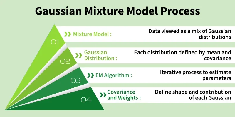
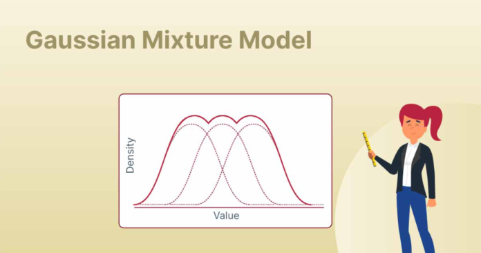
A Gauss mixture model is a probabilistic model that assumes the data is generated from a mixture of several Gaussian distributions. Each Gaussian represents a cluster or component.
Instead of assigning each data point to a single cluster directly, the model assigns probabilities of belonging to each Gaussian component.
Core components of a Gauss mixture model include:
- Mean vectors
- Covariance matrices
- Mixing coefficients
Each component contributes to the overall distribution proportionally to its mixing weight.
Mathematical Foundation of Gaussian Distributions
At the heart of this model lies the Gaussian distribution, also known as the normal distribution.
A Gaussian distribution is defined by:
- Mean, representing the center
- Variance or covariance, representing spread
In one dimension, it forms the familiar bell curve. In higher dimensions, it becomes an ellipsoid defined by a covariance matrix.
The Gauss mixture model combines multiple such distributions to form a more expressive probability density function.
How a Gauss Mixture Model Works

The idea is simple yet powerful.
Each data point is assumed to be generated by one of several Gaussian distributions. However, the identity of the generating distribution is unknown. The model estimates:
- Which Gaussian likely generated each point
- The parameters of each Gaussian
This estimation happens iteratively until convergence.
Instead of rigid cluster boundaries, the model allows soft clustering, meaning one point can partially belong to multiple clusters.
Role of Latent Variables in GMM
Latent variables represent hidden information in the model. In a Gauss mixture model, they indicate which Gaussian component generated each data point.
These variables are not observed directly but inferred during training.
Benefits of latent variables:
- Capture uncertainty
- Enable probabilistic interpretation
- Improve clustering flexibility
This hidden structure is what makes the model powerful for complex datasets.
Expectation Maximization Algorithm Explained
Training a Gauss mixture model relies on the Expectation Maximization algorithm.
Expectation Maximization is an iterative optimization technique used when models depend on latent variables.
It consists of two alternating steps:
- Expectation step
- Maximization step
Each iteration improves parameter estimates until the model converges.
Step-by-Step Working of EM Algorithm
Expectation Step
In this step, the algorithm calculates the probability that each data point belongs to each Gaussian component.
This produces soft assignments instead of hard labels.
Maximization Step
Here, the model updates:
- Means
- Covariances
- Mixing weights
These updates maximize the likelihood of the data given the current assignments.
The steps repeat until changes in likelihood become negligible.
Variants of Gauss Mixture Model
As datasets grow in size and complexity, traditional implementations may face limitations. To address this, several advanced variants of the Gauss mixture model have been developed.
Bayesian Gaussian Mixture Model
A Bayesian version introduces prior distributions over parameters. Instead of fixed values, parameters are treated as random variables.
Benefits include:
- Automatic complexity control
- Reduced overfitting
- Better uncertainty estimation
This approach is especially useful when the true number of clusters is unknown.
Relationship Between Gauss Mixture Model and Density Estimation
One of the most powerful uses of a Gauss mixture model is probability density estimation.
Rather than only clustering, the model learns the entire probability distribution of the data. This allows:
- Sampling new data points
- Detecting anomalies
- Computing likelihoods for unseen observations
In anomaly detection, points with extremely low probability under the learned distribution can be flagged as outliers.
Gauss Mixture Model in High-Dimensional Data
High-dimensional datasets are common in fields like computer vision, genomics, and natural language processing.
Challenges include:
- Increased computational cost
- Covariance matrix instability
- Curse of dimensionality
Practical solutions:
- Dimensionality reduction before modeling
- Diagonal or tied covariance matrices
- Regularization techniques
Combining PCA with a Gauss mixture model is a widely used strategy.
Practical Example: Image Segmentation
In image processing, each pixel can be represented by color intensity values.
A Gauss mixture model can:
- Group pixels based on color similarity
- Segment images into meaningful regions
- Handle gradual color transitions
Unlike threshold-based methods, probabilistic segmentation adapts naturally to noise and lighting variations.
Initialization Techniques in Depth
Initialization is crucial for the success of a Gauss mixture model (GMM). Poor initialization can lead to:
- Convergence to local maxima
- Slow training
- Misleading cluster assignments
Common strategies:
1. Random Initialization
Assign random means and covariances to each Gaussian component.
- Pros: Simple to implement
- Cons: Highly unstable, often requires multiple restarts
2. K-Means Initialization

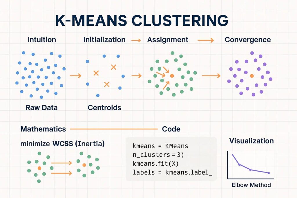
Use K-Means to initialize component means. Covariances are set based on cluster spread.
- Pros: Faster convergence, better results
- Widely used in production systems
3. Hierarchical Initialization
Use hierarchical clustering to determine initial clusters.
- Pros: Can handle non-spherical clusters
- Cons: Computationally expensive
Handling Initialization Sensitivity
Initialization plays a crucial role in convergence quality.
Common initialization techniques:
- Random parameter initialization
- K-Means-based initialization
- Multiple restarts with best likelihood selection
Using K-Means to initialize means often results in faster convergence and better cluster separation.
Computational Complexity Considerations
The computational cost of training depends on:
- Number of data points
- Number of Gaussian components
- Data dimensionality
For large datasets:
- Mini-batch EM
- Approximate inference
- Parallel computation
These techniques help scale the Gauss mixture model to real-world production systems.
Evaluating a Gauss Mixture Model
Proper evaluation ensures your model is accurate and reliable. Methods include:
1. Log-Likelihood
Measures how well the model explains the data. Higher log-likelihood indicates a better fit.
2. Bayesian Information Criterion (BIC)
Penalizes models with more parameters to prevent overfitting.
- Lower BIC = better balance between complexity and fit
3. Akaike Information Criterion (AIC)
Similar to BIC, but less strict in penalizing model complexity.
- Use alongside BIC for robust evaluation
4. Visual Inspection
Plot cluster probability contours or ellipses to verify component separation.
- Useful for low-dimensional datasets
- Helps detect overlapping clusters
Interpretability in Business and Analytics
One reason this model remains popular is interpretability.
Each Gaussian component can be explained as:
- A distinct customer segment
- A behavioral pattern
- A risk profile
This makes it valuable in domains where explainability matters, such as finance, healthcare, and marketing analytics.
Real-World Example of a Gauss Mixture Model
Consider customer spending behavior in an e-commerce platform.
Customers may belong to different purchasing groups:
- Budget shoppers
- Regular buyers
- Premium customers
Their spending data overlaps and cannot be cleanly separated.
A Gauss mixture model can:
- Identify hidden customer segments
- Assign probabilities to each segment
- Support personalized recommendations
This probabilistic insight is far more useful than rigid clustering.
Gauss Mixture Model vs K-Means Clustering
Although both methods are used for clustering, they differ significantly.
K-Means:
- Assigns each point to one cluster
- Assumes spherical clusters
- Uses distance-based logic
Gauss mixture model:
- Allows soft assignments
- Supports elliptical clusters
- Uses probabilistic density estimation
In scenarios with overlapping or non-uniform clusters, a Gauss mixture model performs better.
Applications of Gauss Mixture Model
This model is widely used across industries.
Common applications include:
- Image segmentation
- Speech recognition
- Anomaly detection
- Customer segmentation
- Financial risk modeling
- Density estimation in high-dimensional data
Its flexibility makes it suitable for both academic research and industry solutions.
Common Mistakes to Avoid
When working with a Gauss mixture model, practitioners often encounter pitfalls.
Avoid:
- Using too many components without validation
- Ignoring feature scaling
- Assuming clusters are always meaningful
- Overinterpreting soft probabilities as certainties
Careful validation ensures reliable outcomes.
Comparison With Other Probabilistic Models
Compared to other models:
- Hidden Markov Models add temporal structure
- Kernel density estimation lacks parametric efficiency
- Deep generative models require more data and tuning
A Gauss mixture model remains a balanced choice for many unsupervised learning problems.
Industry Use Cases
Industries using Gauss mixture models include:
- Finance for fraud detection
- Healthcare for patient segmentation
- Retail for demand analysis
- Cybersecurity for anomaly detection
- Autonomous systems for sensor modeling
Its versatility makes it a long-term foundational technique.
Choosing the Number of Components
Selecting the correct number of Gaussian components is critical.
Common techniques include:
- Bayesian Information Criterion
- Akaike Information Criterion
- Cross-validation
Choosing too few components underfits the data, while too many lead to overfitting.
Model Evaluation and Validation
Evaluation focuses on:
- Log-likelihood
- Model stability
- Generalization performance
Visual inspection of clusters and probability contours also helps in understanding model behavior.
Advantages of Using a Gauss Mixture Model
Key benefits include:
- Probabilistic interpretation
- Flexibility in cluster shapes
- Soft clustering capability
- Strong mathematical foundation
These advantages make it a preferred choice for complex data distributions.
Limitations and Challenges
Despite its strengths, the model has limitations.
Challenges include:
- Sensitivity to initialization
- Computational complexity
- Difficulty in selecting component count
Proper preprocessing and parameter tuning are essential for good results.
Practical Implementation Tips
When implementing GMM in Python (scikit-learn):
- Scale Features: Standardize data to avoid dominance of large-magnitude features
- Select Number of Components: Use BIC, AIC, or domain knowledge
- Multiple Initializations: Run EM algorithm multiple times with different seeds
- Monitor Convergence: Ensure likelihood stabilizes to avoid premature stopping
Example snippet:
from sklearn.mixture import GaussianMixture
gmm = GaussianMixture(n_components=3, covariance_type='full', n_init=10)
gmm.fit(X)
labels = gmm.predict(X)
probabilities = gmm.predict_proba(X)
This shows soft clustering probabilities and hard cluster assignments simultaneously.High-Dimensional Data
Tips for Choosing Number of Components
Choosing the correct number of Gaussian components (k) is critical.
- Start with domain knowledge: Estimate clusters based on prior insights
- Evaluate multiple models using BIC/AIC: Select model with lowest score
- Visualize clusters: Check if adding more components improves interpretability
- Cross-validation: Split data into training and test sets for generalization
Practical Implementation Considerations
When implementing a Gauss mixture model:Real-Time Example
- Scale features appropriately
- Initialize parameters carefully
- Monitor convergence
- Validate results using multiple metrics
Libraries such as scikit-learn provide reliable implementations for practical use.
Future Scope of Gauss Mixture Models
Research continues to expand this model through:
- Bayesian Gaussian mixtures
- Variational inference
- Deep generative models
These extensions improve scalability and robustness for modern datasets.
Conclusion
A Gauss mixture model offers a powerful and elegant solution for modeling complex data distributions. By combining probabilistic reasoning with statistical rigor, it enables deeper insights into hidden structures within data.
From customer segmentation to image analysis, this model remains a cornerstone of unsupervised learning. When applied carefully, it delivers interpretability, flexibility, and accuracy that many traditional methods cannot achieve.
Understanding this model equips data professionals with a valuable tool for tackling real-world analytical challenges.
FAQ’s
What is the Gaussian mixture model?
A Gaussian Mixture Model is a probabilistic clustering model that represents data as a combination of multiple Gaussian distributions, commonly used for density estimation and unsupervised learning.
Why is GMM better than Kmeans?
GMM is more flexible than K-Means because it models clusters probabilistically, captures varying shapes and sizes, and provides soft cluster assignments instead of hard labels.
What is the Gaussian mixture model in MIT?
In machine learning, a Gaussian Mixture Model (GMM) is a probabilistic model that represents data as a mixture of multiple Gaussian distributions, often taught in ML courses (including MIT) for clustering and density estimation.
What are the applications of Gaussian mixture models?
Gaussian Mixture Models are used in clustering, density estimation, anomaly detection, image segmentation, speech recognition, and customer behavior modeling, where data follows multiple underlying distributions.
What is the Gaussian model used for?
The Gaussian model is used to represent and analyze data that follows a normal distribution, helping with probability estimation, pattern recognition, statistical inference, and modeling real-world uncertainties.


