Probabilistic Modeling Explained: Hidden Markov Chain in Modern AI Systems

Modern artificial intelligence systems frequently deal with sequential data. Time-series forecasting, speech recognition, and stock market prediction all require models capable of handling temporal dependencies.

One of the most influential statistical frameworks designed for such tasks is the Hidden Markov Chain. It provides a structured probabilistic approach for modeling sequences where the system states are not directly observable.

What Is a Hidden Markov Chain

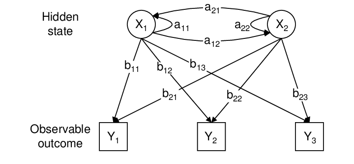
A Hidden Markov Chain is a stochastic process in which:

• The system moves between hidden states
• Each hidden state generates observable outputs
• Transitions follow the Markov property

It is closely related to the Hidden Markov Model, which extends the chain concept to practical probabilistic modeling.

In simple terms:

We observe outputs, but the actual underlying states remain hidden.

Markov Property Explained

The Markov property states:

The probability of the next state depends only on the current state.

Mathematically:

P(Xₙ₊₁ | Xₙ, Xₙ₋₁, …, X₁) = P(Xₙ₊₁ | Xₙ)

This memoryless property simplifies modeling sequential systems.

Example:

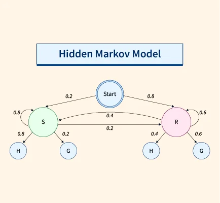
Weather prediction
If today is rainy, tomorrow’s probability depends only on today, not the entire history.

Components of a Hidden Markov Chain

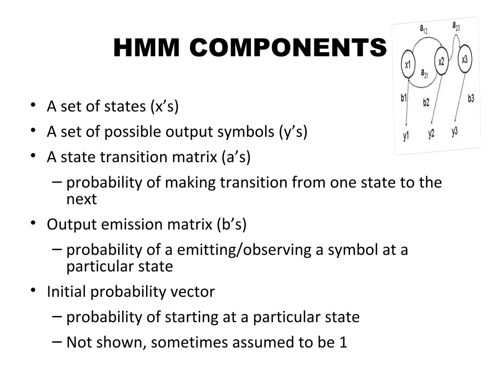
A Hidden Markov Chain consists of:

1. States (Hidden)
2. Observations (Visible)
3. Transition probability matrix
4. Emission probability matrix
5. Initial state distribution

Each component contributes to probabilistic inference.

Mathematical Representation

An HMM is defined by parameters:

λ = (A, B, π)

Where:

A = State transition matrix
B = Emission matrix
π = Initial state distribution

If we have N states:

A = [aᵢⱼ]
Where aᵢⱼ = P(state j at time t+1 | state i at time t)

Emission probability:

bⱼ(k) = P(observation k | state j)

Transition and Emission Probabilities

Transition matrix defines how likely one state moves to another.

Emission matrix defines probability of observing data from a hidden state.

Example:

In speech recognition:

Hidden states = phonemes
Observations = acoustic signals

The Hidden Markov Chain connects sound waves to linguistic units.

Three Fundamental Problems

Hidden Markov Chain modeling revolves around three main problems:

1. Evaluation
   Given model and observations, compute probability of sequence.
2. Decoding
   Find most probable hidden state sequence.
3. Learning
   Estimate model parameters from data.

Forward Algorithm

Used to solve evaluation problem efficiently.

Instead of computing all state combinations, it uses dynamic programming.

Forward probability:

αₜ(j) = P(O₁, O₂, …, Oₜ, state j at time t | λ)

This reduces exponential complexity to polynomial time.

Backward Algorithm

Computes probability from the end of the sequence backward.

Backward probability:

βₜ(i) = P(Oₜ₊₁, …, O_T | state i at time t, λ)

Combining forward and backward improves inference accuracy.

Viterbi Algorithm

Used for decoding.

Finds most likely hidden state sequence.

It uses dynamic programming similar to forward algorithm but maximizes probability instead of summing.

Applications:

• Speech recognition
• Part-of-speech tagging
• DNA sequence alignment

Baum-Welch Algorithm

Used for training.

An Expectation-Maximization (EM) algorithm.

Steps:

E-step
Estimate expected state transitions.

M-step
Maximize likelihood to update parameters.

Iteratively improves Hidden Markov Chain parameters.

Theoretical Foundations of Hidden Markov Chain

While the Hidden Markov Chain is often introduced using simple weather or coin-toss examples, its true power lies in probabilistic graphical modeling and statistical inference.

At a deeper level, a Hidden Markov Chain is a doubly stochastic process:

• One stochastic process governs hidden states
  
• Another governs observed outputs
  

Formally:

Let
S={S₁​,S₂​,…,S_T​} be hidden states
O={O₁​,O₂​,…,O_T​} be observations

The joint probability is:

This structure allows efficient computation using dynamic programming.

Probabilistic Graphical Representation

A Hidden Markov Chain can be represented as a Directed Acyclic Graph (DAG):

S₁ → S₂ → S₃ → … → Sₜ
↓ ↓ ↓
O₁ O₂ O₃

This structure reveals:

• Temporal dependency between hidden states
  
• Conditional independence of observations
  

Observations depend only on their corresponding hidden state.

Likelihood Computation in Depth

Naively computing likelihood involves summing over all possible state sequences:

If there are N states and T time steps:

Total combinations = NT

This becomes computationally intractable.

The Forward Algorithm reduces complexity to:

O(N²T)

This efficiency makes Hidden Markov Chain practical for real-world systems.

Scaling Techniques for Numerical Stability

When dealing with long sequences:

Probabilities become extremely small.

This causes numerical underflow.

Solution:

• Log probability computation
• Scaling factors in forward-backward algorithm

Instead of multiplying probabilities:

Use log-sum-exp trick.

This maintains computational stability.

Continuous vs Discrete Hidden Markov Chain

Discrete HMM

Observations belong to finite categories.

Example:

• Part-of-speech tagging
• DNA sequences

Continuous HMM

Observations are continuous.

Often modeled using Gaussian distributions:

Used in:

• Speech recognition
• Sensor modeling
• Financial forecasting

Hidden Markov Chain and Bayesian Inference

Hidden Markov Chain models align naturally with Bayesian reasoning.

Posterior probability:

P(S_t​∣O)=P(O∣S_t​)P(S_t​)​ / P(O)

Forward-backward algorithm computes posterior distributions efficiently.

This makes HMMs powerful for:

• Sequence smoothing
• State estimation
• Uncertainty modeling

State Duration Modeling

Standard Hidden Markov Chain assumes:

State duration follows geometric distribution.

This is often unrealistic.

Solution:

Hidden Semi-Markov Models (HSMM)

HSMM explicitly models duration distribution.

Applications:

• Speech segmentation
• Human activity recognition
• Medical event modeling

Real-Time Example: Fraud Detection

In online banking:

Observed data:

• Transaction amount
• Location
• Device fingerprint

Hidden states:

• Normal behavior
• Suspicious activity
• Fraudulent state

Hidden Markov Chain detects shifts between normal and fraud regimes.

This improves anomaly detection systems.

Hidden Markov Chain in Natural Language Processing

Before transformers, HMM dominated NLP.

Applications:

• Part-of-speech tagging
• Named entity recognition
• Speech-to-text systems

Viterbi decoding finds most probable tag sequence.

Example:

Sentence:

“AI models optimize systems”

Hidden states:

• Noun
• Verb
• Adjective

HMM determines grammatical structure probabilistically.

Comparing Hidden Markov Chain with Recurrent Neural Networks

Hidden Markov Chain:

• Probabilistic
• Interpretable
• Limited long-term memory

RNN / LSTM:

• Handles long dependencies
• Learns nonlinear transitions
• Requires large datasets

Hybrid systems combine HMM with neural networks.

Example:

Neural-HMM architectures in speech systems.

Parameter Estimation Challenges

Baum-Welch guarantees local optimum.

But:

• Sensitive to initialization
• May converge slowly

Practical solutions:

• Multiple random restarts
• Prior smoothing
• Regularization

Model Selection Criteria

Choosing number of hidden states is critical.

Methods:

AIC (Akaike Information Criterion)
BIC (Bayesian Information Criterion)

These balance:

• Model complexity
• Fit quality

Hidden Markov Chain in Healthcare Analytics

Example:

Monitoring patient vitals.

Observed:

• Heart rate
• Oxygen levels
• Temperature

Hidden states:

• Stable
• Risk
• Critical

HMM predicts patient deterioration earlier than threshold-based methods.

Financial Regime Switching Model

Hidden Markov Chain is widely used for:

• Volatility modeling
• Market regime detection
• Portfolio optimization

Hidden states:

• High volatility
• Low volatility

Investment strategy adapts based on inferred state.

Time Complexity Analysis

Let:

N = number of states
T = sequence length

Forward Algorithm:

O(N²T)

Viterbi Algorithm:

O(N²T)

Baum-Welch:

O(N²T per iteration)

Scales efficiently compared to neural networks.

Practical Python Example

Using hmmlearn:

from hmmlearn import hmm

import numpy as np

model = hmm.GaussianHMM(n_components=3)

X = np.random.rand(100, 1)

model.fit(X)

hidden_states = model.predict(X)

This simple code trains a Hidden Markov Chain on continuous data.

Hidden Markov Chain in IoT Systems

Sensor networks produce sequential data.

Hidden states:

• Machine healthy
• Degrading
• Failure

HMM predicts equipment failure in manufacturing plants.

This supports predictive maintenance.

Integration with Deep Learning

Modern research explores:

Deep Hidden Markov Models (DHMM)

Neural networks parameterize:

• Transition probabilities
• Emission distributions

This combines probabilistic structure with neural flexibility.

Theoretical Perspective: Ergodicity

A Hidden Markov Chain is ergodic if:

• All states communicate
• Long-run state distribution independent of initial state

This ensures stable long-term behavior.

Important for modeling steady systems.

Research-Level Insight

Recent advancements include:

• Variational Hidden Markov Models
• Hierarchical HMM
• Infinite Hidden Markov Models (iHMM)

These extend flexibility and allow adaptive state learning.

Why Hidden Markov Chain Still Matters

Despite deep learning dominance:

• Provides interpretability
• Requires less data
• Computationally efficient
• Strong probabilistic grounding

Understanding Hidden Markov Chain builds a solid foundation for advanced AI.

Hidden Markov Chain in Speech Recognition

Real-time example:

When a user speaks into a voice assistant:

• Acoustic signals captured
• Hidden phoneme states inferred
• Viterbi algorithm decodes most likely word sequence

Hidden Markov Chain was foundational in early speech systems before deep learning.

Applications in Bioinformatics

DNA sequences contain hidden biological states.

Example:

• Exon regions
• Intron regions

Observed sequence = nucleotides
Hidden state = coding or non-coding region

Hidden Markov Chain helps identify gene structures.

Financial Market Modeling

Stock markets exhibit regime changes.

Hidden states:

• Bull market
• Bear market
• Stable market

Observed data:

• Price fluctuations

Hidden Markov Chain detects underlying market regimes.

Comparison with Neural Networks

Hidden Markov Chain:

• Interpretable
• Probabilistic
• Efficient for small data

Neural Networks:

• Data-hungry
• Less interpretable
• More powerful for complex patterns

Modern systems combine both approaches.

Implementation Example in Python

Using hmmlearn library:

Define number of states
Initialize transition matrix
Fit model using observation data

Hidden Markov Chain training is computationally efficient compared to deep neural networks.

Strengths of Hidden Markov Chain

• Strong probabilistic foundation
• Interpretable structure
• Efficient training
• Works well for sequential structured problems

Limitations

• Assumes Markov property
• Limited long-range dependency modeling
• Struggles with highly nonlinear patterns

Deep learning models often outperform in complex tasks.

Conclusion

Hidden Markov Chain remains one of the most elegant probabilistic models in machine learning.

Despite the rise of deep learning, it continues to be relevant in:

• Bioinformatics
• Finance
• Speech processing
• Natural language processing

Understanding Hidden Markov Chain strengthens foundational knowledge in probability theory and sequential modeling.

It bridges classical statistics and modern AI.

FAQ’s