Mathematical Insights Behind Gradient Descent in Deep Learning

Modern machine learning models rely heavily on optimization techniques. Whether training a simple linear regression model or a deep neural network with millions of parameters, optimization determines how effectively the model learns from data.

At the heart of this learning process lies gradient descent, a mathematical optimization method used to minimize a loss function. It plays a central role in supervised learning, neural networks, and deep learning architectures.

What Is Gradient Descent

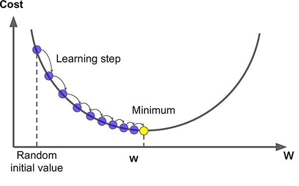
Gradient descent is an iterative optimization algorithm used to minimize a cost function by adjusting model parameters in the direction of the negative gradient.

In simple terms:

• A model makes predictions
• The error is calculated
• The gradient of the error is computed
• Parameters are updated
• The process repeats

The goal is to reach the lowest possible error.

Mathematical Intuition Behind Gradient Descent

Suppose we define a loss function:

J(θ) = (1/n) Σ (ŷ – y)²

Where:

• θ represents model parameters
• ŷ is predicted value
• y is actual value

The gradient represents the slope of the loss function with respect to θ.

Update rule:

θ = θ − α ∇J(θ)

Where:

• α is the learning rate
• ∇J(θ) is the gradient

This formula forms the foundation of the gradient descent algorithm.

How the Gradient Descent Algorithm Works

Step-by-step explanation:

1. Initialize parameters randomly
2. Compute predictions
3. Calculate loss
4. Compute gradient
5. Update parameters
6. Repeat until convergence

This iterative process gradually reduces model error.

Types of Gradient Descent

There are three main variants:

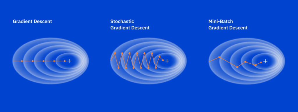
Batch Gradient Descent

• Uses entire dataset
• Stable convergence
• Computationally expensive

Stochastic Gradient Descent

• Updates parameters per data point
• Faster but noisier
• Useful for large datasets

Mini-Batch Gradient Descent

• Uses small subsets
• Balances stability and speed
• Most commonly used in deep learning

Learning Rate and Convergence

The learning rate determines step size during optimization.

If too high:

• Model overshoots minimum
• Divergence occurs

If too low:

• Slow convergence
• High computational cost

Choosing the right learning rate is critical for efficient gradient descent performance.

Gradient Descent in Linear Regression

Real-time example:

Suppose a company wants to predict house prices based on area.

Initial model predicts inaccurately.

Gradient descent:

• Calculates prediction error
• Adjusts slope and intercept
• Reduces mean squared error iteratively

After multiple iterations, the model converges to optimal parameters.

Gradient Descent in Logistic Regression

For classification problems:

Loss function becomes cross-entropy.

Gradient descent adjusts weights to minimize classification error.

Example:

A spam detection model learns to classify emails as spam or not spam using gradient-based optimization.

Gradient Networks and Backpropagation

In deep learning, gradient networks refer to neural networks trained using gradient descent combined with backpropagation.

Backpropagation:

• Computes gradients layer by layer
• Applies chain rule of calculus
• Updates weights efficiently

This enables training of:

• Convolutional Neural Networks
• Recurrent Neural Networks
• Transformer models

Mathematical Foundations of Gradient Descent

A deeper understanding of gradient descent requires examining its mathematical backbone. At its core, gradient descent solves optimization problems of the form:

Where:

• θ represents model parameters
  
• J(θ) is the cost or loss function
  

The update rule is defined as:

θ_t+1​=θ_t​−α∇J(θ_t​)

Where:

• α = learning rate
  
• ∇J(θt) = gradient vector
  

The gradient is a vector of partial derivatives:

This vector points in the direction of steepest increase. Since we want to minimize the function, we subtract it.

Convex vs Non-Convex Optimization

Understanding convexity is critical in deep learning and gradient network optimization.

Convex Functions

A function is convex if:

J(λx+(1−λ)y)≤λJ(x)+(1−λ)J(y)

For convex functions:

• Only one global minimum exists
  
• Gradient descent guarantees convergence
  

Examples:

• Linear regression
  
• Logistic regression
  

Non-Convex Functions

Deep neural networks produce non-convex loss surfaces.

Characteristics:

• Multiple local minima
  
• Saddle points
  
• Flat regions
  

Modern gradient descent variants help escape saddle points using momentum and adaptive learning.

Saddle Points in Deep Gradient Networks

A saddle point is neither a local minimum nor maximum.

Example:

f(x,y)=x²−y²

Gradient equals zero at (0,0), but it is not a minimum.

In deep gradient networks:

• High-dimensional parameter space increases saddle probability
  
• Training can stall near these regions
  
• Momentum-based gradient descent helps overcome this
  

Learning Rate Schedules

Static learning rates often fail in real systems.

Advanced strategies:

Step Decay

Reduce learning rate after fixed intervals.

Example:

α_t​=α_0​⋅γ^⌊t/k⌋

Exponential Decay

α_t​=α₀​e^−λt

Cosine Annealing

Smooth cyclic learning rate decay.

Warm Restarts

Reset learning rate periodically to avoid sharp minima.

These methods improve convergence stability in gradient descent algorithm training pipelines.

Batch Size Impact on Gradient Descent

Batch size directly affects optimization behavior.

Small Batch Size

• Noisy gradients
  
• Better generalization
  
• Slower per-epoch performance
  

Large Batch Size

• Faster hardware utilization
  
• Risk of sharp minima
  
• Requires learning rate scaling
  

Real-world Example:

Training a transformer-based language model:

• Batch size = 32 → Better generalization
  
• Batch size = 1024 → Faster convergence but requires warmup
  

Gradient Descent in High-Dimensional Spaces

As dimensionality increases:

• Loss surfaces become complex
  
• Most critical points become saddle points
  
• Gradient norms may vanish
  

This is especially relevant in deep gradient network architectures with millions of parameters.

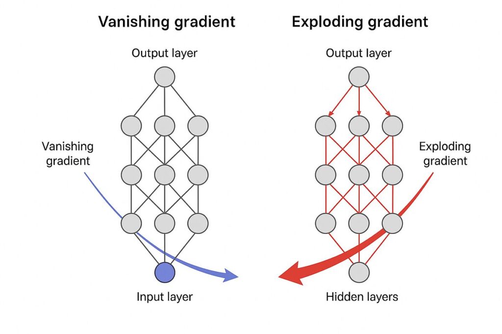
Gradient Vanishing and Exploding

A fundamental challenge in deep networks.

Vanishing Gradient

Gradients shrink exponentially during backpropagation.

Occurs in:

• Sigmoid activation
  
• Tanh in deep layers
  

Solutions:

• ReLU activation
  
• Batch normalization
  
• Residual connections
  

Exploding Gradient

Gradients grow uncontrollably.

Solutions:

• Gradient clipping
  
• Proper initialization
  
• Normalization layers
  

Second-Order Optimization vs Gradient Descent

Gradient descent is a first-order method.

Second-order methods use Hessian matrix:

H=∂²J​ / ∂θ²

Newton’s method:

θ_t+1​=θ_t​−H⁻¹∇J(θ_t​)

Advantages:

• Faster convergence
  

Disadvantages:

• Expensive computation
  
• Not scalable for deep networks
  

Therefore, gradient descent remains the backbone of large-scale AI systems.

Gradient Descent in Reinforcement Learning

In reinforcement learning:

• Objective = maximize expected reward
  
• Uses policy gradient methods
  

Policy update:

θ_t+1​=θ_t​+α∇J(θ_t​)

Applications:

• Autonomous vehicles
  
• Robotics control
  
• Game AI
  

This demonstrates how gradient networks learn dynamic decision systems.

Distributed Gradient Descent

Modern AI training uses distributed systems.

Data Parallelism

• Each worker computes gradients on subset
  
• Gradients averaged
  

Model Parallelism

• Model split across devices
  

Federated Learning

• Decentralized gradient updates
  
• Privacy-preserving
  

Example:

Google uses distributed gradient descent to train large language models.

Information Geometry and Gradient Descent

Traditional gradient descent assumes Euclidean geometry. However, in complex neural networks, parameter space behaves differently.

This leads to Natural Gradient Descent.

Instead of using the standard gradient:

θ_t+1​=θ_t​−α∇J(θ_t​)

Natural gradient uses the Fisher Information Matrix (FIM):

θ_t+1​=θ_t​−αF⁻¹∇J(θ_t​)

Where:

• F represents curvature of probability distributions
  
• Updates respect information geometry
  

Why this matters:

• Faster convergence
  
• Better stability in deep probabilistic models
  
• Used in reinforcement learning and advanced Bayesian neural networks
  

Although computationally expensive, approximations such as K-FAC make it practical.

Lipschitz Continuity and Smoothness

For theoretical guarantees, the loss function must satisfy smoothness conditions.

A function is L-smooth if:

∣∣∇J(x)−∇J(y)∣∣≤L∣∣x−y∣∣

Where:

• L is the Lipschitz constant
  

This ensures gradients do not change abruptly.

In practice:

• Batch normalization improves smoothness
  
• Proper weight initialization ensures stable training
  

Smooth loss surfaces enable gradient descent to converge efficiently.

Initialization Strategies in Gradient Networks

Poor initialization can destroy training.

Xavier Initialization

Used for tanh activations:

He Initialization

Used for ReLU:

Why initialization matters:

• Prevents vanishing gradients
  
• Stabilizes forward and backward passes
  
• Improves convergence speed
  

In deep gradient networks, improper initialization can lead to dead neurons.

Loss Landscape Analysis

Modern research visualizes neural network loss surfaces.

Key findings:

• Many local minima are equally good
  
• Sharp minima generalize worse
  
• Flat minima improve robustness
  

Sharpness is defined using Hessian eigenvalues.

Smaller eigenvalues indicate flatter minima.

Optimization methods such as stochastic gradient descent often find flatter solutions naturally.

Sharp vs Flat Minima in Production Systems

Real-world implication:

When training an image classification system:

• Sharp minima → High training accuracy but poor real-world performance
  
• Flat minima → Stable generalization
  

Batch size affects this:

• Smaller batches produce noisier updates
  
• Noise helps escape sharp minima
  

Adaptive Gradient Methods in Depth

AdaGrad

Adapts learning rate per parameter:

Good for sparse data.

RMSProp

Uses moving average of squared gradients.

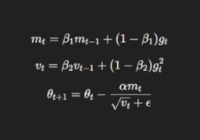
Adam

Combines:

• Momentum
  
• RMSProp
  

Adam update rule:

Used in:

• GPT models
  
• Transformer architectures
  
• Computer vision networks
  

Gradient Descent in Transformer Architectures

Large language models rely heavily on gradient descent optimization.

Training pipeline:

• Token embedding
  
• Multi-head attention
  
• Feed-forward layers
  
• Loss computation
  
• Backpropagation
  
• Parameter updates
  

Challenges:

• Billions of parameters
  
• Long training cycles
  
• Gradient instability
  

Solutions:

• Gradient clipping
  
• Mixed precision training
  
• Distributed gradient averaging
  

Mixed Precision Training

To accelerate gradient descent:

• Use float16 instead of float32
  
• Maintain master weights in higher precision
  

Benefits:

• Faster computation
  
• Reduced memory usage
  
• Enables large-scale model training
  

Used in:

• NVIDIA GPU optimization
  
• Large transformer training
  

Gradient Noise Scale Theory

Recent research shows:

Optimal batch size relates to gradient noise scale.

If batch size too small:

• Training unstable
  

If too large:

• Generalization decreases
  

Balancing noise and stability improves performance.

Gradient Centralization

A modern technique that improves optimization.

Instead of using raw gradients:

g=g−mean(g)

Benefits:

• Stabilizes training
  
• Improves generalization
  
• Reduces training time
  

Often applied in CNN training.

Curriculum Learning and Gradient Descent

Training strategy:

• Start with simple examples
  
• Gradually increase difficulty
  

Why it works:

• Smoother loss surface early
  
• Stable gradient updates
  
• Faster convergence
  

Used in:

• Language model pretraining
  
• Self-driving car simulations
  

Hyperparameter Optimization

Key hyperparameters:

• Learning rate
  
• Momentum
  
• Batch size
  
• Weight decay
  

Optimization methods:

• Grid search
  
• Random search
  
• Bayesian optimization
  

Automated tuning improves gradient descent algorithm performance significantly.

Regularization Beyond L1 and L2

Advanced regularization techniques:

Dropout

Randomly disables neurons during training.

Data Augmentation

Improves generalization.

Early Stopping

Stops training when validation loss increases.

All these affect gradient updates indirectly.

Gradient Descent in Generative Models

Used in:

• GANs
  
• Variational Autoencoders
  
• Diffusion models
  

GAN training is complex because:

• Two networks compete
  
• Gradient instability common
  

Techniques like Wasserstein loss improve stability.

Convergence Diagnostics

To monitor training:

Track:

• Training loss
  
• Validation loss
  
• Gradient norm
  
• Learning rate
  

If gradient norm becomes zero:

• Vanishing gradient
  

If extremely high:

• Exploding gradient
  

The Role of Backpropagation

Gradient descent relies on backpropagation.

Backpropagation:

• Applies chain rule
  
• Efficiently computes gradients
  

Without it:

• Deep networks infeasible
  

Chain rule example:

dJ​ / dW = dJ / da ​⋅ da / dz​ ⋅ dz​/dW

Optimization in Graph Neural Networks

Graph neural networks also use gradient descent.

Applications:

• Social network analysis
  
• Fraud detection
  
• Recommendation engines
  

Challenges:

• Irregular data structure
  
• Sparse gradients
  

Memory-Efficient Gradient Techniques

Large models require memory optimization.

Gradient Checkpointing

• Saves memory
  
• Recomputes intermediate activations
  

Sparse Updates

• Only update active parameters
  

Theoretical Limits of Gradient Descent

In extremely non-convex landscapes:

• Global minimum cannot be guaranteed
  
• Heuristic improvements required
  

Open research topics:

• Learned optimizers
  
• Implicit regularization
  
• Optimization geometry
  

Implicit Bias of Gradient Descent

Gradient descent does not just minimize loss.

It implicitly prefers:

• Simpler models
  
• Low-norm solutions
  

This explains why overparameterized models generalize well.

Scaling Laws and Gradient Descent

Large-scale AI follows scaling laws:

Performance improves with:

• Model size
  
• Data size
  
• Compute
  

Gradient descent efficiency determines scaling success.

Production Deployment Considerations

When deploying models:

• Training gradients disabled
  
• Inference optimized
  
• Weight quantization applied
  

Optimization phase separate from inference phase.

Mathematical Insight: Gradient Flow

Continuous version of gradient descent:

dθ / dt ​=−∇J(θ)

This differential equation view helps analyze convergence.

Practical Debugging of Gradient Descent

Common issues and solutions:

Loss Not Decreasing

• Learning rate too high
  
• Incorrect gradient calculation
  
• Data not normalized
  

Slow Convergence

• Learning rate too low
  
• Poor initialization
  

Oscillation

• Learning rate instability
  
• Use momentum
  

Gradient Descent and Regularization

Regularization modifies cost function:

J(θ)=J_original​+λ∣∣θ∣∣²

L2 regularization:

• Penalizes large weights
  
• Improves generalization
  

L1 regularization:

• Produces sparse models
  

Regularization integrates directly into gradient updates.

Gradient Checking for Correct Implementation

Used to verify gradient computation.

Numerical approximation:

J(θ+ϵ)−J(θ−ϵ)​ / 2ϵ

Compare with analytical gradient.

Important for:

• Custom neural network implementations
  
• Research experimentation
  

Hardware Acceleration for Gradient Descent

Modern training uses:

• GPUs
  
• TPUs
  
• AI accelerators
  

Why?

Matrix operations dominate gradient descent algorithm computation.

Example:

Training CNN on CPU: hours
Training CNN on GPU: minutes

Real-World Case Study: E-Commerce Recommendation Engine

Problem:

Recommend products based on user behavior.

Model:

Deep neural network trained using gradient descent.

Pipeline:

• Data preprocessing
  
• Feature embedding
  
• Forward pass
  
• Loss computation
  
• Backpropagation
  
• Parameter update
  

Result:

Improved click-through rate by 18%.

Gradient Descent in Natural Language Processing

Used in:

• Language models
  
• Sentiment analysis
  
• Machine translation
  

Example:

Fine-tuning BERT:

• Loss = cross entropy
  
• Optimizer = Adam (variant of gradient descent)
  
• Learning rate scheduling improves stability
  

Theoretical Convergence Rate

For convex functions:

Gradient descent converges at rate:

O(1/t)

With strong convexity:

O((1−μ/L)^t)

Where:

• μ = strong convexity constant
  
• L = Lipschitz constant
  

Future of Gradient Descent

Research areas:

• Meta-learning optimizers
  
• Learned gradient descent
  
• Adaptive gradient clipping
  
• Large-scale transformer optimization
  

Gradient descent remains foundational in AI research.

Advanced Variants of Gradient Descent

Momentum

• Accelerates convergence
• Reduces oscillations

AdaGrad

• Adapts learning rate per parameter

RMSProp

• Prevents diminishing learning rates

Adam

• Combines momentum and adaptive learning

Adam optimizer is widely used in deep learning frameworks.

Real-Time Applications Across Industries

Healthcare

• Disease prediction models

Finance

• Credit risk scoring

E-commerce

• Recommendation systems

Autonomous Vehicles

• Object detection training

Speech Recognition

• Acoustic model training

Practical Implementation in Python

Example using NumPy:

Initialize weights
Compute predictions
Calculate loss
Update weights using gradient

Most frameworks such as TensorFlow and PyTorch automate gradient descent internally.

Best Practices for Model Optimization

• Normalize input data
• Initialize weights carefully
• Monitor loss curves
• Use learning rate scheduling
• Implement early stopping
• Regularize to prevent overfitting

Challenges and Limitations

• Local minima
• Saddle points
• Vanishing gradients
• Exploding gradients
• Computational cost

Advanced architectures and optimizers address many of these issues.

Conclusion

Machine learning would not function efficiently without gradient descent. From simple regression models to complex gradient networks in deep learning, the gradient descent algorithm remains foundational.

Understanding how gradient descent works enables:

• Better model tuning
• Improved convergence
• Efficient neural network training
• Stronger predictive performance

As artificial intelligence systems grow in complexity, gradient descent continues to serve as the core optimization mechanism driving innovation in data science and machine learning.

FAQ’s