When building machine learning models, one of the biggest challenges is finding the best parameters to minimize prediction errors. This is where gradient descent becomes a core optimization algorithm.
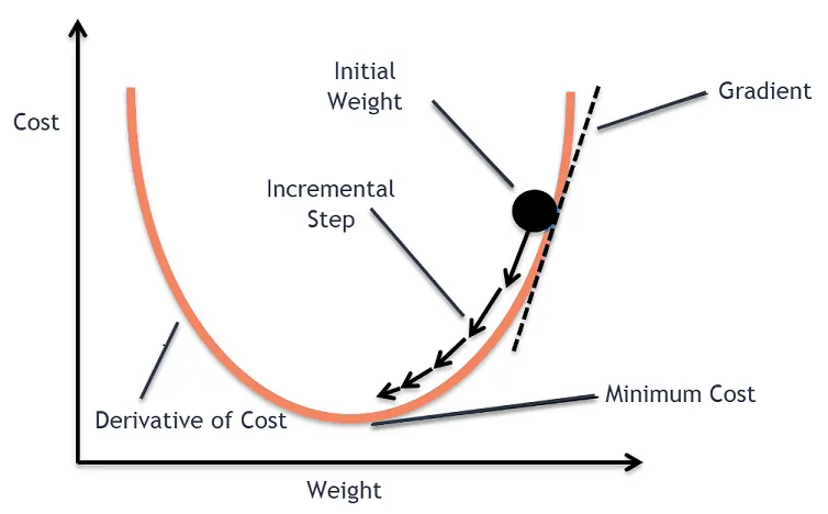
Instead of randomly guessing model weights, gradient descent systematically moves toward the minimum of the cost function, adjusting parameters to achieve better performance.
Think of it like hiking down a mountain in the fog — you can’t see the entire path, but by taking careful steps in the steepest downward direction, you eventually reach the valley.
What is Gradient Descent
Gradient Descent is an optimization algorithm used in machine learning to find the set of parameters that minimize a model’s error. Instead of guessing the best values, the algorithm moves step-by-step in the direction where the cost function decreases the fastest. This movement is guided by the gradient, which acts like a slope showing the steepest downward direction. By iteratively updating parameters, Gradient Descent helps models learn patterns, reduce prediction errors, and achieve better accuracy across tasks such as regression, classification, and deep learning.
What is a Loss Function
A Loss Function measures how far the model’s predictions are from the actual target values. It quantifies the error for a single training example, indicating whether the model is performing well or poorly. When the loss is low, predictions are close to the truth; when it is high, the model needs improvement. Loss functions are the foundation of optimization because Gradient Descent uses them to compute gradients and adjust parameters. Examples include Mean Squared Error for regression and Cross-Entropy Loss for classification.
What is a Cost Function
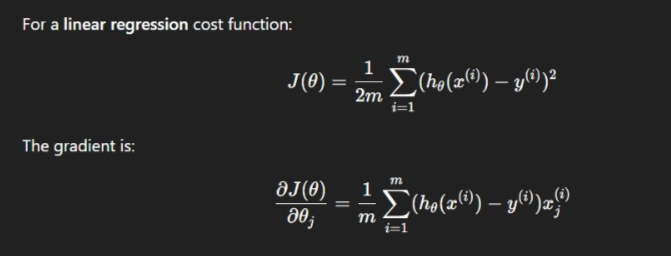
A Cost Function represents the overall error of the model across the entire training dataset. It aggregates the individual losses into a single value, helping determine how well the model fits the data. Gradient Descent works by minimizing this cost function, making it central to the training process. A lower cost value means the model achieves better generalization and makes more accurate predictions. Common cost functions include the average error across all samples, such as Mean Squared Error in linear regression.
Why Gradient Descent Matters in Machine Learning
Gradient descent is the backbone of many algorithms, from linear regression to deep neural networks. It’s not just a mathematical trick — it’s a practical method for:

- Training models efficiently even with massive datasets.
- Minimizing loss functions to improve accuracy.
- Adapting weights automatically without human intervention.
- Scaling algorithms to work in high-dimensional spaces.
Example:
In image recognition, models need to adjust millions of parameters. Gradient descent automates this, making the learning process feasible and efficient.
Batch Gradient Descent for Machine Learning
Batch Gradient Descent calculates the gradient of the cost function using the entire dataset at once. Because it considers every training sample, it provides highly accurate gradient updates, allowing the model to steadily approach the global minimum. However, this accuracy comes with the trade-off of slower computation, especially on large datasets. Batch Gradient Descent is most effective when the dataset is small to medium-sized or when computational resources are strong enough to process all samples simultaneously.
Stochastic Gradient Descent for Machine Learning
Stochastic Gradient Descent (SGD) updates model parameters using only one data point at a time, making it significantly faster and more efficient for large datasets. Its frequent updates introduce noise into the optimization path, causing it to zig-zag rather than move smoothly downhill. Although this makes convergence less stable, the randomness helps the algorithm escape local minima and reach better solutions. SGD is widely used for deep learning and real-time applications where speed and scalability are critical.
How Gradient Descent Works – Step-by-Step

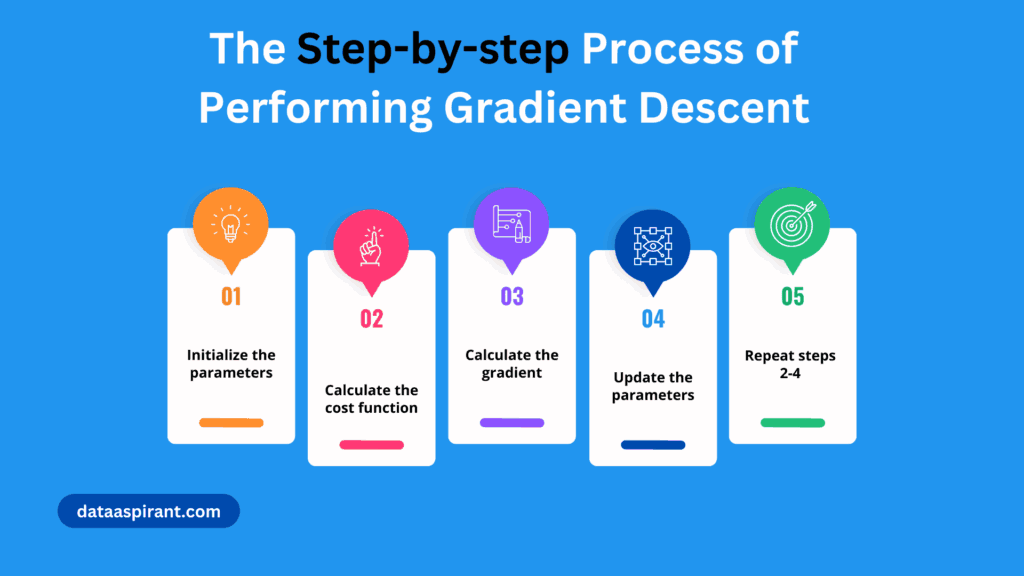
Here’s a simple breakdown:
- Initialize Parameters: Start with random weights.
- Compute the Gradient: Calculate how much the cost function changes for each parameter.
- Update Parameters: Move in the opposite direction of the gradient (downhill).
- Repeat: Keep updating until the model converges to the optimal solution.

Key Variants of Gradient Descent
Gradient descent comes in multiple flavors, each with pros and cons:
A. Batch Gradient Descent
- Uses the entire dataset to compute gradients.
- Accurate but slow for large datasets.
B. Stochastic Gradient Descent (SGD)
- Updates weights after each training example.
- Faster but noisier convergence.
C. Mini-Batch Gradient Descent
- Compromise between batch and SGD.
- Common in deep learning.
D. Momentum-based Gradient Descent
- Adds momentum to speed up convergence and avoid local minima.
E. Adaptive Methods (Adam, RMSProp, Adagrad)
- Adjust learning rates dynamically for each parameter.
Mathematical Foundation of Gradient Descent
Gradient descent is rooted in calculus and optimization theory. The gradient is the vector of partial derivatives that points in the direction of the steepest ascent. To minimize a function, we move against this direction.

The Geometry of Gradient Descent
At its core, Gradient Descent is a geometric transformation in high-dimensional space. Each parameter update shifts the model’s position in the loss landscape, which can be thought of as a complex surface filled with valleys, peaks, and saddle points. Unlike simple convex functions, deep learning models operate in non-convex loss surfaces with millions of dimensions. While these landscapes contain many local minima, research shows that most are “good minima,” meaning they generalize well. The real challenge lies in saddle points—flat regions where gradients approach zero, slowing convergence. Techniques like Momentum and Adam help escape such regions faster.
The Role of Hessian Matrix and Second-Order Insights
While Gradient Descent uses the first derivative, more advanced optimization methods analyze the Hessian matrix, which contains second-order partial derivatives. The Hessian describes the curvature of the cost function:
- Positive curvature → the algorithm is approaching a minimum
- Negative curvature → near a maximum
- Zero curvature → saddle point
Second-order methods like Newton’s Method converge faster but are computationally expensive for deep learning due to the enormous size of the Hessian. This is why first-order methods like SGD remain dominant.
Learning Rate Schedules and Adaptive Strategies
Modern deep learning rarely uses a static learning rate. Instead, dynamic learning rate strategies accelerate convergence and prevent overfitting.
Popular learning rate strategies:
- Step Decay – learning rate reduces after fixed epochs
- Exponential Decay – decreases continuously as training progresses
- Warm Restarts (SGDR) – cyclic learning rate that periodically resets
- Cosine Annealing – smooth learning rate transitions for stable convergence
These schedules allow the model to explore the loss landscape early and fine-tune efficiently in later training phases.
Gradient Descent with Regularization
Gradient Descent often incorporates regularization to balance accuracy and generalization.
Common regularization techniques:
- L1 Regularization (Lasso): adds sparsity by shrinking certain weights to zero
- L2 Regularization (Ridge): penalizes large weights to stabilize training
- Dropout: randomly drops neurons, forcing the network to rely on multiple patterns
Regularization modifies the cost function, meaning the gradient now includes both error reduction and penalty terms.
Gradient ClippingIn deep neural networks, especially RNNs and LSTMs, gradients can explode, causing weights to increase uncontrollably.
Gradient Clipping restricts the gradient’s magnitude, preventing unstable updates.
This is critical for training stable sequence models, NLP architectures, and transformer-based networks.
Real-World Examples and Use Cases
Gradient descent is everywhere in machine learning:
- Natural Language Processing (NLP): Optimizing embeddings in Word2Vec or BERT.
- Computer Vision: Training convolutional neural networks for image classification.
- Recommender Systems: Adjusting weights for user-item interaction predictions.
- Financial Forecasting: Optimizing time-series models.
Example: In self-driving cars, neural networks trained with gradient descent detect pedestrians and traffic signals by minimizing classification errors.
Challenges and Limitations
Even though gradient descent is powerful, it’s not perfect:
- Local Minima: Can get stuck in non-optimal points.
- Learning Rate Selection: Too high causes overshooting; too low causes slow convergence.
- Feature Scaling Issues: Requires normalization for faster convergence.
- Computational Cost: Large datasets require significant processing power.
Tips for Improving Gradient Descent Performance
To get the most from gradient descent:
- Normalize data before training.
- Choose a suitable learning rate — try learning rate schedules.
- Use mini-batches for faster computation.
- Add momentum to avoid local minima.
- Experiment with adaptive optimizers like Adam.
Visualizing Gradient Descent
Is one of the most effective ways to understand how this optimization algorithm works in practice. By plotting the cost function against the model parameters, we can observe how the algorithm iteratively moves towards the minimum point. In a 2D view, this often appears as a smooth curve where the gradient descent steps take the parameter values downhill, reducing the error at each iteration. In higher dimensions, contour plots or surface plots are used to show the optimization path, often visualized as a zig-zagging or spiraling trajectory towards the optimal point.
These visualizations make it easier to grasp the effects of the learning rate—too high, and the algorithm overshoots; too low, and it converges slowly. Real-time animations, available through tools like Matplotlib in Python, can help track each step and reveal whether the algorithm is stuck in local minima or progressing steadily to the global minimum.
A contour plot or 3D surface plot is often used to visualize how parameters move toward the optimum.
For example, in Python (Matplotlib + NumPy), you can animate the descent to see how weights adjust over iterations.
Image Alt Text Example:
“Visualization of gradient descent optimization process over a cost function surface.”
Tips for Gradient Descent
To achieve the best performance with Gradient Descent, it’s essential to choose an appropriate learning rate—too high may cause divergence, while too low leads to slow training. Normalizing or standardizing input features helps the algorithm converge more efficiently by maintaining balanced parameter scales. Mini-batches offer a good compromise between speed and stability, making them ideal for deep learning. Using techniques such as momentum, learning rate decay, and adaptive optimizers like Adam can further accelerate convergence and improve accuracy.
Real-World Applications of Gradient Descent
Gradient Descent plays a vital role in almost every modern machine learning task. In computer vision, it optimizes millions of parameters in convolutional neural networks for image recognition. In natural language processing, it powers the training of embeddings and transformers like BERT and GPT. Businesses rely on Gradient Descent to build recommender systems, forecasting models, fraud detection systems, and predictive analytics engines. Even fields like autonomous driving, healthcare diagnostics, and finance depend on Gradient Descent to fine-tune complex AI models that must learn from massive datasets.
External Tools and Resources for Learning Gradient Descent
- TensorFlow Optimizers Documentation
- PyTorch Optim Module
- Gradient Descent Visualization Tool
TensorFlow Playground, Google Colab, and Kaggle Notebooks provide interactive environments to experiment with gradient descent and visualize its optimization process. Online courses, tutorials, and documentation from platforms such as Coursera, Analytics Vidhya, and Scikit-learn further help in building a deeper theoretical and practical understanding.
Final Thoughts
Gradient descent is the workhorse of machine learning optimization.
From simple regression to cutting-edge deep learning models, it enables efficient training and accurate predictions.
By mastering gradient descent — understanding its math, variants, and real-world applications — you gain a solid foundation for building smarter and faster AI systems.
FAQ’s
How gradient descent is used for optimization?
Gradient descent optimizes a model by iteratively adjusting parameters in the direction of the steepest decrease of the loss function, allowing the model to gradually minimize errors and improve performance.
Why use gradient descent instead of ols?
Gradient descent is preferred over OLS when datasets are large, high-dimensional, or involve complex models where computing the OLS closed-form solution becomes too slow or computationally expensive.
Does Adam Optimizer use gradient descent?
Yes, the Adam optimizer is an advanced variant of gradient descent that uses adaptive learning rates and momentum to achieve faster and more stable convergence during training.
What are the three types of gradient descent?
The three types of gradient descent are Batch Gradient Descent, Stochastic Gradient Descent (SGD), and Mini-Batch Gradient Descent, each differing in how much data they use to compute gradients during optimization.
What is an example of gradient descent?
A common example of gradient descent is training a linear regression model, where the algorithm iteratively adjusts the slope and intercept to minimize the mean squared error between predicted and actual values.


