Random Forest vs Decision Tree: The Ultimate Power Guide to Smarter Machine Learning Models

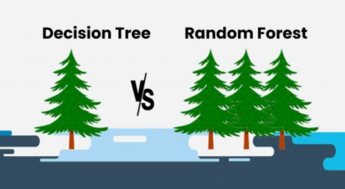
In the world of machine learning, Random Forest vs Decision Tree is one of the most frequent comparisons analysts, data scientists, and AI professionals encounter. Both models are powerful in their own ways—Decision Trees for their interpretability and simplicity, and Random Forests for their robustness and superior predictive accuracy.

The question is: When should you use one over the other?
This comprehensive guide explores every dimension of these models — theory, mathematics, practical examples, business use cases, and even Python code — to help you make the right choice.

Understanding Decision Tree

What Is a Decision Tree?

A Decision Tree is a supervised learning algorithm used for both classification and regression tasks. It represents data using a tree-like model of decisions and possible consequences.

Each internal node represents a feature (attribute), each branch represents a decision rule, and each leaf node represents the outcome.

How Decision Trees Work

1. The algorithm splits the dataset into subsets based on the value of input features.
   
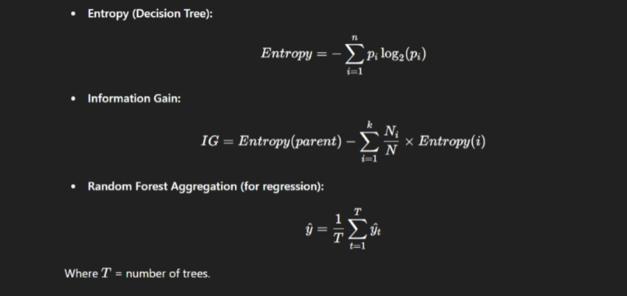
2. The best split is chosen using metrics like:
   
   • Gini Impurity (CART)
     
   • Information Gain (ID3/C4.5)
     
3. This process continues recursively until all samples are classified perfectly or stopping conditions are met.

Real-World Example of Decision Trees

Consider a telecom company predicting customer churn based on:

• Monthly Charges
  
• Contract Type
  
• Tenure
  
• Internet Service Type

A Decision Tree might first split on Contract Type, then on Monthly Charges, leading to interpretable decision paths like:

“If Contract = Month-to-Month and Monthly Charges > 70, then Customer is likely to churn.”

Understanding Random Forest

What Is a Random Forest?

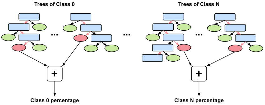
A Random Forest is an ensemble learning technique that builds multiple Decision Trees and merges their results for improved accuracy and stability.

It operates on the principle of Bagging (Bootstrap Aggregation) — training each tree on random subsets of data and features.

How Random Forest Works

1. Bootstrap Sampling: Random subsets of data are drawn (with replacement).
   
2. Random Feature Selection: Each tree is trained using a random subset of features.
   
3. Voting/Averaging: Predictions from all trees are combined:
   
   • Majority vote (classification)
     
   • Average (regression)

Real-World Example of Random Forest

A Random Forest used for loan approval prediction might build 200 different trees, each trained on slightly different samples of data. When combined, these models yield a highly stable and accurate prediction, reducing overfitting.

Random Forest vs Decision Tree: The Core Difference

Feature	Decision Tree	Random Forest
Nature	Single model	Ensemble of multiple trees
Overfitting	High	Low
Accuracy	Moderate	High
Interpretability	High	Moderate
Computation Time	Fast	Slower
Bias-Variance Trade-off	High variance	Reduced variance
Robustness	Sensitive to data changes	Stable due to averaging

In essence, Random Forest = Many Decision Trees + Randomness + Aggregation.

Mathematical Foundation Behind Both Models

Pros and Cons: Random Forest vs Decision Tree

Decision Tree Advantages

• Easy to interpret and visualize.
  
• Requires little data preprocessing.
  
• Works for both categorical and continuous data.

Decision Tree Disadvantages

• Prone to overfitting.
  
• Unstable with small data variations.

Random Forest Advantages

• Excellent generalization and accuracy.
  
• Reduces overfitting through averaging.
  
• Handles missing values efficiently.

Random Forest Disadvantages

• Difficult to interpret.
  
• Requires more computational resources.

Hyperparameter Tuning for Random Forest and Decision Tree

Parameter	Description	Impact
max_depth	Maximum depth of trees	Prevents overfitting
min_samples_split	Minimum samples for a split	Controls tree growth
n_estimators (RF)	Number of trees	More trees = better performance
max_features (RF)	Number of features per split	Adds randomness

Example (Python):

from sklearn.ensemble import RandomForestClassifier

model = RandomForestClassifier(n_estimators=100, max_depth=8, random_state=42)

model.fit(X_train, y_train)

When to Use Random Forest vs Decision Tree

• Use Decision Tree for interpretability, quick insights, or small datasets.
  
• Use Random Forest for large, noisy datasets requiring accuracy and generalization.

Handling Overfitting: Why Random Forest Wins

Decision Trees can perfectly memorize training data, leading to poor test accuracy.
Random Forests prevent this by averaging predictions from multiple uncorrelated trees, minimizing variance and improving generalization.

Random Forest vs Decision Tree in Modern Machine Learning

While Decision Trees and Random Forests are classic algorithms, they have evolved significantly with advancements in computational power, distributed systems, and the rise of interpretability-driven AI. Understanding these deeper aspects helps data professionals make better architectural and operational decisions.

Advanced Performance Considerations

1. Computational Complexity

• Decision Tree Complexity:
  
  • Training: O(n×m log⁡ n) where n = samples, m = features
    
  • Space: Moderate, as only one model is stored
    
  • Prediction: Very fast due to single path traversal
    
• Random Forest Complexity:
  
  • Training: O(T×n×m log⁡ n), where T = number of trees
    
  • Space: Higher (storing hundreds of trees)
    
  • Prediction: Slower due to ensemble aggregation

While Decision Trees can train in seconds, Random Forests may take minutes or hours depending on n_estimators and data size.

2. Parallelization and Scalability

Random Forests, despite being computationally expensive, are highly parallelizable. Each tree can be trained independently, making it suitable for:

• Multi-core CPUs
  
• GPU-accelerated frameworks
  
• Distributed systems like Apache Spark MLlib or Dask

Decision Trees, being single models, are less suited for parallelization but ideal for real-time systems or resource-constrained environments.

Handling Imbalanced and High-Dimensional Data

1. Class Imbalance

When dealing with datasets where one class dominates (e.g., fraud detection), Random Forests can:

• Use class_weight = ‘balanced’
  
• Combine with SMOTE (Synthetic Minority Over-sampling Technique) for synthetic data generation

Decision Trees, however, may become biased toward majority classes unless tuned properly with weighted Gini or Entropy.

2. High-Dimensionality

Random Forests perform automatic feature selection due to random feature subsetting, making them robust in high-dimensional problems such as:

• Text classification (TF-IDF vectors)
  
• Genomic data analysis
  
• Sensor fusion tasks

Decision Trees tend to overfit or become unstable when dealing with thousands of correlated features.

Interpretability: Bridging the Black Box

One major criticism of Random Forests is their lack of transparency. However, several modern techniques have emerged to make them interpretable:

1. Feature Importance Analysis

Feature importance in Random Forests can be measured by:

• Mean Decrease in Gini Impurity
  
• Permutation Importance
  
• SHAP (SHapley Additive exPlanations) values for local interpretability

Example:

import shap

explainer = shap.TreeExplainer(model)

shap_values = explainer.shap_values(X_test)

shap.summary_plot(shap_values, X_test)

This visualization shows how each feature influences the prediction at a granular level — bridging the interpretability gap between Random Forest and Decision Tree.

2. Surrogate Modeling

A surrogate Decision Tree can be trained on the predictions of a Random Forest to approximate its decision boundaries.
This approach enables business stakeholders to interpret Random Forests through a simpler, human-readable model.

Advanced Variants and Hybrids

Researchers and data engineers have proposed several enhancements over traditional Random Forests and Decision Trees to handle modern data challenges.

1. Extra Trees (Extremely Randomized Trees)

• Introduced randomness not just in feature selection but also in split thresholds
  
• Faster training
  
• Less overfitting
  
• Slightly less accurate than traditional Random Forests in some datasets

2. Rotation Forests

Combines Principal Component Analysis (PCA) with Random Forest to rotate feature space, enhancing diversity between trees and improving classification accuracy.

3. Gradient Boosted Decision Trees (GBDTs)

Unlike Random Forests that average independent trees, GBDTs (like XGBoost, LightGBM, CatBoost) build trees sequentially — each new tree corrects errors of the previous one.

Key difference:

• Random Forest: Parallel trees, bagging
  
• GBDT: Sequential trees, boosting

4. Oblique Decision Trees

Use linear combinations of features at each split instead of single features. These trees handle correlated features better and improve decision boundaries in high-dimensional spaces.

Statistical Generalization and Bias-Variance Trade-off

Both algorithms address the bias-variance trade-off differently:

Model	Bias	Variance	Error Behavior
Decision Tree	Low bias	High variance	Overfits on training data
Random Forest	Slightly higher bias	Low variance	Stable predictions

The ensemble averaging in Random Forest reduces variance substantially while maintaining a low bias, making it more robust across unseen data.

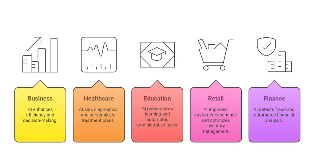
Real-World Applications Beyond Traditional Machine Learning

1. Healthcare

• Decision Trees help clinicians trace logical pathways to diagnosis.
  
• Random Forests power high-accuracy models for predicting disease risks (e.g., diabetes or heart disease).

2. Climate and Environmental Science

Random Forests handle non-linear, noisy datasets, such as predicting air quality or rainfall based on multiple environmental variables.

3. Finance

Decision Trees are used for credit rule creation, while Random Forests handle fraud detection, loan default prediction, and algorithmic trading signals.

4. Retail

E-commerce platforms use Random Forests for recommendation systems, customer segmentation, and dynamic pricing models.

5. Cybersecurity

Random Forests identify anomalies in real-time, detecting malicious network behavior and intrusion attempts.

Advanced Tuning and Optimization Strategies

1. Hyperparameter Optimization Techniques

Manual tuning is inefficient for large models. Modern optimization frameworks like:

• Optuna
  
• Hyperopt
  
• Bayesian Optimization
  automatically search the best combination of hyperparameters.

Example (using Optuna):

import optuna

def objective(trial):

    n_estimators = trial.suggest_int('n_estimators', 100, 1000)

    max_depth = trial.suggest_int('max_depth', 3, 20)

    model = RandomForestClassifier(n_estimators=n_estimators, max_depth=max_depth)

    model.fit(X_train, y_train)

    return model.score(X_valid, y_valid)

2. Out-of-Bag (OOB) Error Estimation

Random Forests provide an internal cross-validation metric — OOB error — calculated on data not used in bootstrap samples, saving computational cost.

Model Interpretability vs Predictive Power Trade-off

In enterprise AI pipelines, this trade-off is crucial:

• Decision Tree: Ideal for explainable AI requirements (e.g., banking compliance)
  
• Random Forest: Ideal for high-stakes prediction systems where performance matters most

Organizations often use both:

• Decision Tree for decision auditability
  
• Random Forest for operational prediction accuracy

Handling Missing and Noisy Data

Random Forest inherently manages missing values by:

• Using surrogate splits
  
• Imputing missing features based on majority class
  
• Averaging predictions across trees

Decision Trees require preprocessing, but modern implementations (like in scikit-learn 1.4+) can handle NaNs directly.

Research and Emerging Trends (2024–2030)

1. Federated Random Forests

• Enable privacy-preserving learning by training distributed Random Forests across devices without sharing raw data.
  
• Used in healthcare, finance, and IoT.

2. Quantum Decision Forests

• Quantum computing-based variants that drastically reduce tree-building time and improve decision boundary exploration.

3. Explainable Random Forests (XRF)

• New frameworks integrating rule extraction and SHAP explanations to make ensemble models fully interpretable.

4. Hybrid Deep Forest Models

• Combine neural networks and forest algorithms, where Random Forest outputs feed into deep layers for nonlinear representation learning.

5. AutoML Integration

• Automated Machine Learning (AutoML) platforms (like Google Cloud AutoML and H2O AutoML) increasingly use Random Forests as baseline models due to their balance between accuracy and interpretability.

Comparative Summary: Beyond Traditional Metrics

Dimension	Decision Tree	Random Forest
Speed (Training)	Very fast	Moderate
Speed (Prediction)	Instant	Slower
Interpretability	Excellent	Moderate
Robustness	Poor under noise	Strong
Scalability	Limited	High
Feature Correlation Handling	Weak	Moderate
Data Imbalance Handling	Weak	Strong
Suitability for Real-Time	High	Low
Model Deployment Size	Lightweight	Heavy
Explainability in Regulated Industries	Excellent	Limited

Feature Importance Comparison

Both models offer feature importance, but Random Forest averages importance across all trees, providing more reliable insight.

Example output (in Python):

import pandas as pd

importance = pd.Series(model.feature_importances_, index=features)

importance.sort_values(ascending=False)

Real-Time Example: Predicting Customer Churn

Dataset Features:

• Tenure
  
• Monthly Charges
  
• Internet Service
  
• Payment Method

Decision Tree Accuracy: ~82%
Random Forest Accuracy: ~91%

This clearly demonstrates how Random Forests outperform single trees in generalization and stability.

Visualization Comparison

• Decision Tree: Tree diagram with feature splits.
  
• Random Forest: Aggregated forest representation — not visually simple but statistically robust.

Key Metrics for Evaluation

• Accuracy
  
• Precision / Recall / F1 Score
  
• ROC-AUC
  
• Confusion Matrix

Use:

from sklearn.metrics import classification_report

print(classification_report(y_test, y_pred))

Integration with Python (Code Snippets)

Decision Tree Example:

from sklearn.tree import DecisionTreeClassifier

clf = DecisionTreeClassifier(max_depth=5)

clf.fit(X_train, y_train)

Random Forest Example:

from sklearn.ensemble import RandomForestClassifier

rf = RandomForestClassifier(n_estimators=200)

rf.fit(X_train, y_train)

Common Mistakes to Avoid

• Not tuning hyperparameters.
  
• Using Random Forest with too few trees.
  
• Ignoring feature scaling.
  
• Misinterpreting feature importance.

Random Forest and Decision Tree in Business Applications

• Finance: Fraud detection, credit scoring
  
• Healthcare: Disease prediction, patient risk modeling
  
• Retail: Customer segmentation, recommendation systems
  
• Manufacturing: Defect prediction and quality analysis

Advanced Concepts: Ensemble Learning and Bagging

Ensemble Learning combines multiple weak learners to form a strong learner.
Bagging (Bootstrap Aggregation) ensures randomness, diversity, and reduced variance — core to Random Forest success.

External Tools and Libraries

• Scikit-learn (Python)
  
• H2O.ai
  
• TensorFlow Decision Forests
  
• XGBoost (for gradient-boosted trees)

Conclusion

In the debate of Random Forest vs Decision Tree, both algorithms play vital roles depending on context.

• If interpretability and simplicity matter, Decision Tree wins.
  
• If prediction accuracy and robustness are the goal, Random Forest is unbeatable.

In real-world machine learning pipelines, both are often complementary — Decision Trees for exploration, Random Forests for deployment.

FAQ’s