Autocorrelation Decoded: A Powerful and Insightful Guide for Time Series Analysis

Modern data rarely exists in isolation. Many datasets evolve gradually, influenced by past values and historical conditions. Examples include stock prices, daily temperature readings, website traffic, energy demand, and sensor-generated signals.

These datasets share a common structure: time dependency. Understanding how present observations relate to past values is critical for building reliable analytical and predictive systems. Without acknowledging this structure, insights can become misleading and decisions unreliable.

Why Time Dependency Changes Data Interpretation

Traditional statistical models often assume independence between observations. Time-based data violates this assumption by nature.

Ignoring temporal relationships can result in:

• Inflated confidence levels
  
• Incorrect hypothesis testing
  
• Overestimated model performance
  
• Poor forecasting accuracy
  

This is why specialized time series techniques exist, designed to capture internal patterns that evolve across time.

Understanding Autocorrelation Conceptually

At its core, autocorrelation measures how strongly a variable is related to itself across different points in time. Instead of comparing two separate variables, the comparison happens within the same variable, but at different time lags.

This helps answer a fundamental analytical question:

Does the past influence the present in a measurable way?

The answer determines whether future behavior can be anticipated or if the data behaves randomly.

Mathematical Foundations Behind Temporal Dependence

Consider a sequence of daily electricity consumption values. If today’s usage closely resembles yesterday’s, then the series shows a strong internal relationship.

Such dependence can arise from:

• Behavioral habits
  
• Physical constraints
  
• Economic cycles
  
• Environmental persistence
  

Understanding these patterns provides insight into how stable or volatile a system truly is.

Autocorrelation Formula Explained Step by Step

The autocorrelation formula quantifies the similarity between observations separated by a fixed time lag.

Explanation of Components

• X_t: value at time t
  
• Xˉˉ: mean of the entire series
  
• k: time lag
  
• n: total observations
  

The output ranges between −1 and +1, indicating direction and strength of dependence.

Role of Lag in Time Series

Lag defines how far apart two observations are in time.

Examples include:

• Lag one: today compared to yesterday
  
• Lag two: today compared to two days earlier
  
• Lag seven: today compared to last week
  

Different lag values reveal different structural behaviors in data.

Autocorrelation Function and Its Purpose

The autocorrelation function calculates autocorrelation values across a sequence of lags instead of focusing on a single lag.

This provides a complete temporal dependency profile of a dataset.

Why It Matters

• Detects seasonality
  
• Identifies persistence
  
• Supports model selection
  
• Reveals randomness or structure
  

How to Read and Interpret an ACF Plot

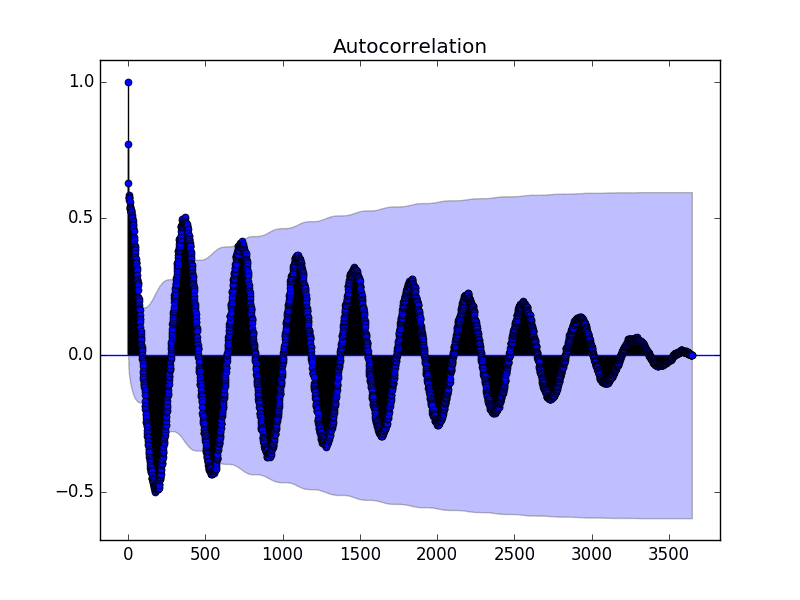
An ACF plot displays correlation strength on the vertical axis and lag on the horizontal axis.

Interpretation guidelines:

• Slowly decreasing bars indicate long-term dependence
  
• Repeating spikes suggest seasonal behavior
  
• Rapid drop toward zero indicates weak memory
  
• Values within confidence bounds imply randomness

Partial Autocorrelation and Why It Matters

While the autocorrelation function measures total dependence between observations at different lags, it does not isolate direct relationships. This limitation becomes important when multiple lagged effects overlap.

Partial autocorrelation solves this problem by measuring the direct correlation between a variable and a specific lag, while removing the influence of intermediate lags.

Why Partial Autocorrelation Is Important

• Helps identify the true order of autoregressive processes
  
• Prevents misleading lag interpretation
  
• Improves forecasting model selection
  
• Clarifies causal structure in time-based systems
  

In practice, analysts use partial autocorrelation plots alongside ACF plots to determine appropriate model complexity.

Relationship Between Autocorrelation and Partial Autocorrelation

Aspect	Autocorrelation Function	Partial Autocorrelation
Measures	Total dependency	Direct dependency
Includes indirect effects	Yes	No
Used for	MA model selection	AR model selection
Visualization	ACF plot	PACF plot

Using both together provides a clearer picture of temporal structure.

Statistical Tests for Autocorrelation

Visual inspection is not always sufficient. Formal tests help determine whether observed dependency is statistically significant.

Commonly Used Tests

Durbin–Watson Test
Primarily used in regression residuals to detect first-order dependence.

Ljung–Box Test
Evaluates whether a group of autocorrelations is jointly zero.

Breusch–Godfrey Test
Detects higher-order autocorrelation in regression models.

These tests are especially important in econometrics and hypothesis-driven research.

Autocorrelation in Regression Residuals

In regression analysis, residuals are expected to be independent. When autocorrelation appears in residuals, it indicates that the model has failed to capture important temporal structure.

Consequences include:

• Biased standard errors
  
• Invalid confidence intervals
  
• Incorrect hypothesis tests
  

Addressing this issue is critical for reliable inference.

How to Fix Autocorrelation in Models

Several techniques exist to correct or reduce temporal dependence.

Common Solutions

• Differencing the dependent variable
  
• Adding lagged variables
  
• Using autoregressive error models
  
• Applying generalized least squares
  
• Switching to time-series-specific models
  

The choice depends on the nature and source of dependence.

Seasonal Autocorrelation Explained

Seasonality introduces repeating patterns at fixed intervals. This results in strong autocorrelation at seasonal lags.

Examples include:

• Weekly traffic patterns
  
• Monthly sales cycles
  
• Annual climate fluctuations
  

Seasonal differencing is often required to handle such patterns effectively.

Autocorrelation and Forecast Horizon

Short-term forecasts often benefit strongly from autocorrelation, while long-term forecasts depend more on structural trends and external variables.

Key insights include:

• Strong short-lag dependence improves near-term predictions
  
• Long-range forecasts require trend modeling
  
• Over-reliance on past values reduces adaptability
  

Understanding this balance is essential for operational forecasting.

Autocorrelation in Signal Processing

In signal processing, autocorrelation helps identify repeating signals buried in noise.

Applications include:

• Speech recognition
  
• Radar signal detection
  
• Audio processing
  
• Pattern extraction
  

It enables systems to recognize structure even in noisy environments.

Autocorrelation in Control Systems

Control systems rely on temporal feedback loops. Autocorrelation analysis helps determine system stability and response time.

Use cases include:

• Manufacturing automation
  
• Robotics
  
• Power grid management
  
• Industrial monitoring
  

Detecting excessive dependence can prevent oscillations and instability.

Autocorrelation and Long-Memory Processes

Some time series exhibit long-term dependence where correlations decay very slowly.

Examples include:

• Internet traffic
  
• Financial volatility
  
• Climate indices
  

Such behavior requires specialized models like fractional differencing.

Interpreting Weak Autocorrelation

Weak autocorrelation does not always imply randomness. External drivers, structural breaks, or regime changes can suppress internal dependence.

Analysts should consider:

• External covariates
  
• Policy changes
  
• Market interventions
  
• Environmental shocks
  

Context is essential for correct interpretation.

Autocorrelation in Deep Learning Time Models

Recurrent neural networks and transformer-based models implicitly learn autocorrelation patterns.

However:

• Overfitting can amplify noise
  
• Lack of interpretability hides dependence structure
  
• Explicit analysis improves trust and debugging
  

Combining statistical diagnostics with deep learning improves robustness.

Autocorrelation and Anomaly Detection

Sudden changes in temporal dependency often indicate anomalies.

Examples include:

• Equipment failure
  
• Fraudulent transactions
  
• Cyber intrusions
  
• Environmental disasters
  

Monitoring changes in autocorrelation patterns enables early warning systems.

Practical Workflow for Time Series Dependency Analysis

A recommended workflow includes:

• Visualizing the raw series
  
• Checking stationarity
  
• Plotting ACF and PACF
  
• Running statistical tests
  
• Selecting appropriate models
  
• Validating using rolling forecasts
  

This structured approach reduces analytical errors.

Advanced Python Example Including Partial Autocorrelation

from statsmodels.graphics.tsaplots import plot_acf, plot_pacf

import matplotlib.pyplot as plt

plot_acf(data, lags=40)

plot_pacf(data, lags=40)

plt.show()

This dual visualization clarifies both total and direct dependence.

Real-World Examples Across Industries

Business Demand Forecasting

Retail sales often depend on previous demand patterns, promotional cycles, and holidays.

Industrial Sensor Monitoring

Machine vibrations or temperature readings often show persistence until maintenance occurs.

Social Media Engagement

Post interactions tend to follow daily and weekly cycles driven by user behavior.

Autocorrelation in Financial Markets

In finance, autocorrelation is used to analyze:

• Market efficiency
  
• Volatility clustering
  
• Momentum and mean reversion
  

Price returns may appear random, while volatility often shows strong persistence.

Autocorrelation in Weather and Climate Science

Weather variables exhibit strong temporal structure due to physical laws.

Applications include:

• Climate trend detection
  
• Seasonal forecasting
  
• Extreme event modeling
  

Ignoring time dependence in climate data can lead to incorrect conclusions.

Autocorrelation in Digital and Web Analytics

Website traffic, session duration, and conversion rates often follow repeatable temporal patterns.

Use cases include:

• Server capacity planning
  
• Campaign performance evaluation
  
• User behavior analysis
  

Positive, Negative, and Zero Dependence

Positive Dependence

Values tend to follow previous trends.

Negative Dependence

Values oscillate or reverse direction.

Zero Dependence

Values behave like random noise with no memory.

Difference Between Correlation and Autocorrelation

Aspect	Correlation	Autocorrelation
Variables	Two different	Same variable
Time	Ignored	Explicit
Use Case	Cross-sectional	Time-based

Stationarity and Its Impact

Stationarity implies stable statistical properties over time.

Non-stationary data often exaggerates dependency and must be corrected using:

• Differencing
  
• Log transformations
  
• Seasonal adjustment
  

Autocorrelation in Predictive Modeling

Autoregressive models explicitly rely on internal temporal relationships.

Common examples:

• AR
  
• ARIMA
  
• Seasonal ARIMA
  

The autocorrelation function helps determine appropriate model structure.

Machine Learning Considerations

Many machine learning algorithms assume independent samples.

Ignoring temporal dependence may cause:

• Data leakage
  
• Overestimated accuracy
  
• Poor real-world performance
  

Time-aware validation strategies are essential.

Implementation Using Python

from statsmodels.graphics.tsaplots import plot_acf

import matplotlib.pyplot as plt

plot_acf(data, lags=30)

plt.show()

This visualization is a standard first step in time series exploration.

Common Mistakes and Misinterpretations

• Treating dependence as causation
  
• Ignoring non-stationarity
  
• Over-interpreting minor spikes
  
• Using inappropriate confidence bounds
  

Best Practices for Reliable Analysis

• Always visualize dependency
  
• Test for stationarity
  
• Use domain knowledge
  
• Validate with time-based splits
  

When Temporal Dependence Helps

• Forecasting future values
  
• Detecting anomalies
  
• Understanding system behavior
  
• Designing control mechanisms
  

When Temporal Dependence Causes Issues

• Regression assumption violations
  
• Inflated statistical significance
  
• Misleading inference

Corrective techniques include generalized least squares and differencing.

Final Thoughts and Key Takeaways

Understanding how past values influence present behavior is essential in modern analytics. Autocorrelation provides a structured framework to quantify this relationship, making it indispensable for time series analysis.

By mastering the formula, interpreting the autocorrelation function, and applying best practices, analysts can unlock deeper insights and build more reliable predictive systems across industries.

FAQ’s